ADOMETA
- ADoption
of Orphan METabolic Activities
|
||
The Challenge |
||
Accurate reconstruction of metabolic networks is essential to understanding the biochemical organization of sequenced organisms. Homology-based methods can now annotate a significant fraction of metabolic genes in a given organism. However, even the state-of-the art homology methods cannot annotate sequences with no or little sequence identity to known enzymes. This resulted in orphan metabolic activities - metabolic reactions without any responsible sequences. We can classify orphan metabolic activities to be locally or globally orphan (Osterman and Overbeek 2003, Karp 2004). Global orphan activities do not have a single representative sequence in any organism. In contrast, local orphan activities represent reactions for which we do not have a representative sequence in a given organism, although one or several sequences catalyzing the reaction may be known in other organisms. Because of various reasons, major metabolic databases and models do not always agree upon enzymatic functional annotations. Thus the situation occurs that sometimes one metabolic activity is deemed to be locally orphan in a specific organism based on one model while not the other. Nevertheless, a simple calculation reveals that the number of global orphan activities is substantial. Also a list of global orphan activities as of Feb 2006 can be found here. In recent years, so-called genomic context based methods, such as phylogenetic profile, mRNA co-expression profile, gene clustering and protein fusion have shown promising points in recovering metabolic networks, particularly for sequences with little or no sequence similarity to any known sequences. We believe that the combination of the homology and context-based methods will enhance our ability of identifying genes for orphan activities trememdously. Towards this goal have been developing a bioinformatics resource named ADOMETA, ADOption of Orphan METabolic Activities, as part of the research projects in the Vitkup Laboratory at Columbia University. ADOMETA currently provides computationally generated predictions of genes for orphan activities in the model bacteria Escherichia coli and B. subtilis as well as the baker's yeast S. cerevisiae. |
||
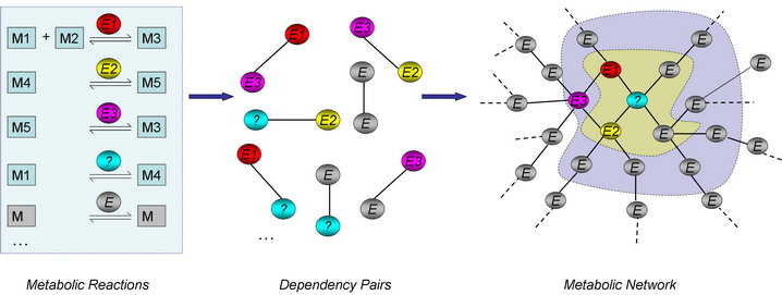
Metabolic networks are represented by the metabolic gene connectivity graph. The nodes of the graph correspond to metabolic genes, and the edges correspond to the dependencies (connections) established by metabolic reactions (See the figure below). Metabolic genes X and Y will be connected if the corresponding proteins share a common metabolite among their reactants or products.
The construction of a metabolic network from a list of metabolic reactions and visualization of a “network gap” (orphan activity). Abbreviations: M: Metabolite; E: Enzyme. Metabolites serve as edges in the network and enzymes as nodes. The orphan activity or “metabolic gap” is designated by “?” and surrounded by known metabolic genes. We refer the "first layer neighbors" (yellow in the figure) of a target gene to describe the collection of genes with distance one to the target gene, "second layer neighbors" (grey in the figure) to describe genes with distance two and so on. |
||
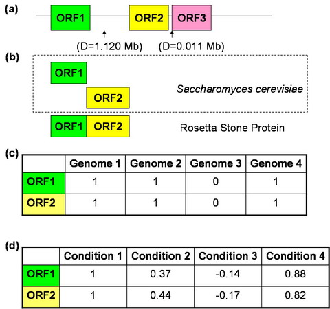
Several context-based correlations were successfully introduced previously (Enright et al., 1999; Huynen and Bork, 1998; Marcotte et al., 1999; Pellegrini et al., 1999). Context-based correlations between genes establish a similarity in the selective pressures during evolution. This similarity allows one to infer a functional connection. The following graph shows the idea.
(a) The gene clustering method identifies genes closely located on a chromosome. (b) The Rosetta Stone method identifies gene fusion events between homologs of a gene pair in other organisms. (c) The phylogenetic profiles method identifies genes which tend to co-occur together in different genomes. (d) The method based on the similarity of genes co-expression across different conditions.Genes with similar functions tend to co-express. |
||
Context-based Signals in a Metabolic Network |
||
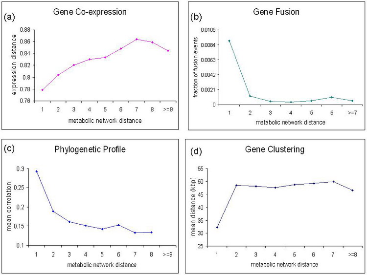
It is important to understand if context-based signals are strong enough to determine the exact network location of a hypothetical gene. The established metabolic network allows us to quantify the relationship between the gene distance in the network and the average genomic context-based information. In the figure (S. cerevisiae) below we show correlations of different context-based methods between a target gene and all other network genes separated from the target by distance one, two, three, and so on. For all types of the context-based methods, we see a clear trend of monotonical decreasing (or increasing) relationship between the context-based correlation and metabolic network distance (Chen et al).
The figure above shows different types of context-based associations versus the metabolic network distance for the S. cerevisiae metabolic network: (a) Gene
co-expression (DeRisi
et al., 1997; Wu
et al., 2002). Numerous studies demonstrated that genes with similar
mRNA co-expression profiles usually have related functions. Co-expression
distances were calculated as |1-Spearman’s rank correlation|
between co-expression profiles for a given organism, for example,
E. coli, B. subtilis or S. cerevisiae. E. coli
co-expression profiles were obtained from the Stanford Microarray Database
(Ball,
2005). S. cerevisiae co-expression profiles were obtained from
the Rosetta “compendium” dataset (Hughes
et al., 2000). B. subtilis co-expression information were transferred
from E. coli orthologous genes, which was determined by using
BLAST (Altschul
et al., 1997) best bi-directional search. Other types of genomic context-based associations, such as gene distance (measuring physical distance between genes on the chromosome of the genome of interest) are not plotted on the figure but it shows the same trend. Additionally although no network structure exists in annotated pathways, it is oftentimes benificial to consider the context-based correlations between a candidate gene and known pathway genes. Genes that are highly correlated with known pathway genes are more likely to carry out a reaction (sometimes a gap) in that particular pathway. The pathway distance descriptor measure the shortest chromosomal distance of a candidate gene to any known genes in the pathway that the target activity is involoved. |
||
General Strategy to Adopt an Orphan Activity using Context Data |
||
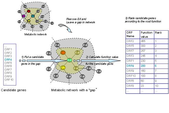
The conceptual idea of the our approach is illustrated in the figure below. The fit of a particular gene for a network gap is determined by the strength of functional correlations with known genes close to the gap. The context-based methods are used to calculate the functional correlations. The strength of the fit is determined by fitness (cost) functions such as the one listed below: |
||
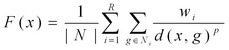 |
where x is the candidate gene, |N| is the total of number genes contributing to the fitting, R is the maximal layer around the gap contributing to the fitness function, Ni is the set of genes in i-th layer (1st, 2nd, 3rd, etc.) around the gap, d(x,g) is a context-based correlation between genes x | |
and the gap g, wi is a weight determining the relative contribution of the different layers, p is a positive factor determining how the decrease in a context-based correlation should decrease the contribution to the fit. In the function, the first summation is for all the genes of a certain network layer around the gap, the second summation is for each contributing layer. For more information about cost functions, please see Kharchenko et al. and Chen et al.The performance of our fitting procedure can be quantified by the fraction of correct genes ranked - based on the fitness function - as the top 1 or within the top 10 genes out of a large collection of unrelated genes (for example more than 6,000 non-metabolic genes in S. cerevisiae). These ranks are shown separately in the prediction table.
Testing a set of candidate genes for the fit into a network gap (orphan metabolic activity). The genes from the candidate set are tested one by one and the fit is determined by a fitness function (see Chen et al.). The function values are higher for candidates with good context-based correlations to the genes neighboring the gap. Based on the fitness function values the genes are ranked (right column of the figure). We use the following self-consistent procedure to evaluate performance of the method: Each known gene is removed from the network – leaving a gap in its place - and the gene rank is calculated among all non-metabolic genes (>6,000 genes for yeast) for the created gap. This procedure is repeated for all known metabolic genes. The method performance is quantified by the fraction of the correct genes ranked as the top (corresponding to P value < 1.6*10-4) or within the top 10 (P value < 1.6*10-3) out of all non-metabolic genes. |
||
| Homology information | ||
All candidate genes were aligned against the Swissprot Database (Bairoch and Apweiler, 2005) sequences to obtain homology scores using BLAST searches. Two types of scores were recorded: (a) Best
Sequence Idenity to Proteins Assigned the full EC number of interest
(SEQ4) is calculated as the best sequence identity
score to all known Swissprot
enzymes (excluding enzymes from the investigated organism) assigned
the EC number of interest. For example, if the EC number of interest
is “4.1.3.30”, the best sequence identity of a candidate
gene to all Swissprot enzymes annotated as “4.1.3.30” is
recorded as SEQ4 (“4” means it is specific to ALL 4 digits
of EC). Sequence identity scores obtained were considered valid if the
corresponding alignment has an E-value of at least 2e-5. We use the
very loose E-value in that we intend to use even the most remote homology.
If, for example, no sequence homology was detected between a candidate
gene and any Swissprot enzymes
assigned the EC number of interest, "0" and "20"
are assigned as the SEQ4 and E-value, respectively. |
||
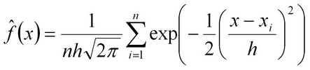
Currently, we use the MLjava implementaion of the AdaBoost algorithm and Alternating Decision Tree (ADT) developed by Dr. Freund et al (Ref 1, 2, 3) to combine genomic context-based associations and sequence homology score into a single accurate predictor. We plan to use several additional strategies to integrate different types of associations in the near future. The "Overall Rank" presented in the prediction table represents the overall strength of evidence that a candidate gene may be responsible for a particular orphan activity of interest.We assess the confidence in each predictions by calculating the tail probability (P-value) of each score. To do so, we need a reliable estimate of the distribution of scores under the null hypothesis, which is the assumption that the gene’s product does not catalyze the metabolic reaction we are interested in. For a given metabolic gap, the scores of virtually all candidate genes can be regarded as samples taken from the background distribution, as most genes do not encode the enzyme for that particular enzymatic activity. Hence, we can estimate the background distribution under the null hypothesis from the set of scores of all candidate genes for a particular metabolic gap. In practice, we found that this distribution does not resemble either a normal distribution or an extreme-value distribution, rendering a P-value estimation from such a fitted distribution inaccurate. Instead, having a large sample of background scores for each gap allows us to use the kernel density estimation method (Silverman, Density Estimation for Statistics and Data Analysis, 1986, Chapman and Hall, New York) (Scott, Multivariate Density Estimation; Theory, Practice, and Visualization, 1992, John Wiley and Sons, New York), which can estimate a distribution non-parametrically. For a Gaussian kernel, the estimated background distribution is
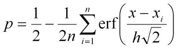
In contrast to parametrically estimated distribution functions, the kernel estimate of the P-value takes the distance between the top score and runner-up scores directly into account. If the score x is much larger than all other scores xi, the error function approaches unity, and the P-value will be small. On the other hand, if the top score is attained by several genes, each of them will contribute a term 1/2n to the P-value. E-value or the expected value takes into account the size of the candidate gene sets and is calculated simply as the P-value multiplied by the number of candidate genes in a particular gene set. |
||